Bounding-Box Inference for Error-Aware Model-Based Reinforcement Learning

Talvitie, Erin J., et al. “Bounding-Box Inference for Error-Aware Model-Based Reinforcement Learning.” Reinforcement Learning Conference, 2024.

Info

I replicated the results presented in this paper. The codebase can be found in this GitHub repository (in python).

The original codebase for the paper can be found in this GitHub repository (in C++).

warning

This content is a summary and includes my personal takeaways from the paper "Bounding-Box Inference for Error-Aware Model-Based Reinforcement Learning" by Talvitie et al. It reflects the points I found most relevant, along with my own conclusions on the topics discussed.

For a more comprehensive understanding of the topics and to align with the authors' perspectives, please READ THE PAPER.

Introduction

Model-Based Reinforcement Learning (MBRL) aims to learn a model of the environment dynamics to reduce sample complexity and potentially improve policy performance. Let

$$\mathcal{M} = (\mathcal{S}, \mathcal{A}, p, r, \gamma)$$

be a Markov Decision Process (MDP), where $\mathcal{S}$ is the state space, $\mathcal{A}$ is the action space, $p(s'|s,a)$ is the transition distribution, $r(s,a)$ is the reward function, and $\gamma \in [0,1]$ is the discount factor. The goal is to find a policy $\pi(a|s)$ that maximizes the expected discounted return

$$G_t = \sum_{i=0}^{\infty} \gamma^i R_{t+i+1}.$$

In MBRL, the agent simultaneously learns a model $(\hat{p}, \hat{r})$ that approximates $(p, r)$ and uses it to simulate state-action transitions. Naively treating simulated rollouts as ground truth can mislead the value function and degrade the policy. This problem is particularly acute when the model has insufficient capacity, when the hypothesis space is inadequately explored, or when training samples are limited.

The paper defines:

• Aleatoric uncertainty as the inherent randomness in the environment. This uncertainty is irreducible—no amount of additional data or model refinement can eliminate it.

• Epistemic uncertainty as the uncertainty over the model parameters due to limited data. Unlike aleatoric uncertainty, epistemic uncertainty is reducible through additional data.

• Model inadequacy as the error arising from a model’s structural limitations or oversimplifications. This type of uncertainty cannot be fully resolved merely by acquiring more data; it requires a fundamental revision of the model.

Selective planning aims to mitigate catastrophic planning by weighing model-based value targets according to their estimated reliability.

The paper uses the Model-based Value Expansion (MVE), which computes multi-step targets:

$$\hat{\rho}_1 = r_{t+1} + \gamma \max_{a'}\hat{q}(S_{t+1}, a'),$$

and for $h>1$,

$$\hat{\rho}_h = r_{t+1} + \sum_{i=2}^{h}\gamma^{i-1}\hat{r}_{t+i} + \gamma^h \max_{a'} \hat{q}(\hat{S}_{t+h}, a'),$$

where $(\hat{s}_{t+i}, \hat{r}_{t+i})$ are generated by the model. By weighting these targets based on uncertainty, selective planning can exploit accurate predictions while ignoring harmful ones.

The paper present a novel uncertainty measure for MVE—Bounding-Box Inference (BBI). BBI infers upper and lower bounds on the multi-step targets and weights them according to the gap between these bounds.

Problem Setting and Mathematical Formulation

We consider an MDP with unknown dynamics $p$ and reward $r$. At each time $t$, the agent observes a state $S_t \in \mathcal{S}$, selects an action $A_t \in \mathcal{A}$, and receives a reward $R_{t+1}=r(S_t,A_t)$. The environment transitions to a new state $S_{t+1} \sim p(\cdot|S_t,A_t)$.

The agent maintains a state-action value function $\hat{q}(s,a)$ to approximate

$$q_{*}(s,a) = \max_\pi q_{\pi}(s,a),$$

where

$$q_{\pi}(s,a) = \mathbb{E}[\sum_{i=0}^{\infty}\gamma^i R_{t+i+1}|S_t=s,A_t=a,\pi].$$

The agent also learns a model $(\hat{p}, \hat{r})$ approximating $p$ and $r$.

Selective MVE Update

Let $w_h \geq 0$ be the weight assigned to the $h$-step target. The selective MVE update is given by:

$$\hat{q}(S_t,A_t) \leftarrow \hat{q}(S_t,A_t) + \alpha\left(\sum_{h=1}^H\frac{w_h \hat{\rho}_h}{\sum_{h'=1}^H w_{h'}}- \hat{q}(S_t,A_t)\right).$$

Let $u_h$ be the uncertainty measure associated with horizon $h$. We form weights via a softmin:

$$w_h = \frac{\exp(-u_h/\tau)}{\sum_{j=1}^H \exp(-u_j/\tau)},$$

where $\tau>0$ is a temperature parameter. As $\tau \rightarrow 0$, the update approaches Q-learning; as $\tau \rightarrow \infty$, it approaches uniform weighting.

The challenge is to define the uncertainty over the simulated targets, $\hat{\rho}_h$.

Uncertainty Measures

Several uncertainty measures are compared in the paper:

1. One-Step Predicted Variance (1SPV):
   1SPV estimates uncertainty by aggregating the predicted variances of one-step model predictions over the rollout. Specifically, the uncertainty at horizon $h$ is given by:

   $$u_h = \sum_{j=0}^{h-1} \left( \sum_d \hat{\sigma}_d^2(s_{t+j}, a_{t+j}) + \hat{\sigma}_r^2(s_{t+j}, a_{t+j}) \right)^2,$$

   where $\hat{\sigma}_d^2(s, a)$ represents the predicted variance of the next state dimension $d$, and $\hat{\sigma}_r^2(s, a)$ represents the predicted variance of the reward at state $s$ and action $a$. Although computationally efficient, this method can be overly conservative when state uncertainties do not translate directly to uncertainty in TD targets.

2. Monte Carlo Target Variance (MCTV):

   This approach estimates uncertainty by sampling $k$ rollouts from the model for the same initial transition. Given samples $\{\hat{\rho}^j_h\}_{j=1}^k$ at horizon $h$, the mean target is defined as:

   $$\hat{\rho}_h = \frac{1}{k} \sum_{j=1}^k \hat{\rho}^j_h,$$

   and the uncertainty is estimated as the sample variance:

   $$u_h = \frac{1}{k-1} \sum_{j=1}^k (\hat{\rho}^j_h - \hat{\rho}_h)^2.$$

   This method directly estimates uncertainty over TD targets, though its accuracy depends on the number of samples and the model’s predicted distribution.

3. Monte Carlo Target Range (MCTR):

   Instead of using variance, MCTR defines uncertainty as the range of the sampled targets:

   $$u_h = \max_j \hat{\rho}^j_h - \min_j \hat{\rho}^j_h.$$

   This measure directly captures the spread of possible outcomes and is less sensitive to assumptions about the distribution’s shape, though it still depends on the number of samples.

4. Bounding-Box Inference (BBI):

   BBI uses a bounding-box over states and actions to infer upper and lower bounds on the TD targets. Consider a bounding-box over states $\overline{\underline{s}} = [\underline{s}, \overline{s}]$ and over actions $\overline{\underline{a}}$. Define:

   $$\underline{q}(\overline{\underline{s}}_t,\overline{\underline{a}}_t) = \inf_{s\in\overline{\underline{s}}_t,a\in\overline{\underline{a}}_t}\hat{q}(s,a), \quad \overline{q}(\overline{\underline{s}}_t,\overline{\underline{a}}_t)=\sup_{s\in\overline{\underline{s}}_t,a\in\overline{\underline{a}}_t}\hat{q}(s,a).$$

   Similarly, given the current state and action $(S_t,A_t)$ and the actual next transition $(S_{t+1}, R_{t+1})$, we define a bounding-box model rollout:

   $$\overline{\underline{r}}_{t+i}, \overline{\underline{s}}_{t+i}, \overline{\underline{a}}_{t+i}, \quad \text{for } i=2,\dots,h.$$

   The bounding-box TD target at horizon $h$:

   $$\underline{\rho}_h = R_{t+1} + \sum_{i=2}^h \gamma^{i-1}\underline{r}_{t+i} + \gamma^h \underline{v}(\overline{\underline{s}}_{t+h}),$$ $$\overline{\rho}_h = R_{t+1} + \sum_{i=2}^h \gamma^{i-1}\overline{r}_{t+i} + \gamma^h \overline{v}(\overline{\underline{s}}_{t+h}),$$

   where $\overline{v}(\overline{\underline{s}}) = \max_{a \in \overline{\underline{a}}} \overline{q}(\overline{\underline{s}},a)$ is the maximum possible value with the states and actions included. And $\underline{v}(\overline{\underline{s}}) = \max_a \underline{q}(\overline{\underline{s}},a)$ is the least you can get with the states and actions included.

   The BBI uncertainty is $u_h = \overline{\rho}_h - \underline{\rho}_h$. This approach is distribution-insensitive and relies on conservative bounding, ensuring that no harmful scenario is overlooked. Though potentially conservative, BBI avoids catastrophic failures due to model misestimation.

Empirical Evaluation

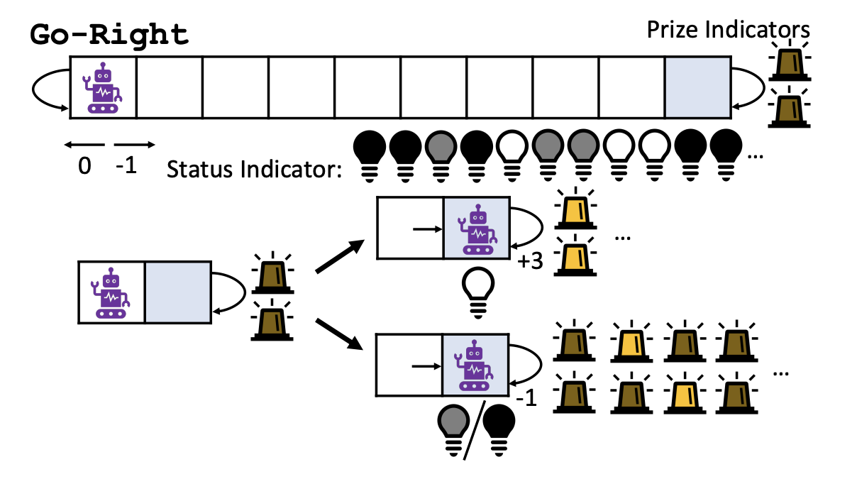
The paper evaluates uncertainty‐aware selective planning using the GoRight environment, which is designed to test exploration and planning under model error.

GoRight Environment

In the GoRight environment, the objective is to reach the rightmost position under specific conditions. The state consists of:

1. Position:

   • Integer $\{0, \dots, 10\}$.
   • Observed as a float with an offset in $[-0.25, 0.25]$.
   • Actions left, right shift the agent’s position by $\pm 1$.

2. Status Indicator ($\{0,5,10\}$):

   • Observed with an offset $\in [-1.25,1.25]$.
   • Follows a deterministic 2nd-order Markov pattern (defined by a transition table in the paper).
   • If the agent enters position 10 while this status is at 10, the prize condition is triggered.

3. Prize Indicators ($\{0,1\}$):

   • Two indicators in standard GoRight, or ten in GoRight10.
   • Observed with offsets $\in[-0.25,0.25]$.
   • They are all 0 outside position 10; they turn fully 1 (all on) only when the agent has successfully hit the prize condition (see status indicator). Otherwise, when the agent is in position 10 but has not triggered the prize, the lights cycle in a fixed pattern (all off, then only the first turns on, then only the second, and so on)

4. Rewards:

   • 0 for a left action.
   • -1 for a right action unless the agent is in position 10 with all prize indicators = 1, in which case the right action yields +3.

Although the underlying dynamics are discrete, the agent receives noisy, continuous observations. This noise makes the environment partially observable; in particular, the agent does not have access to the previous status indicator value, so a perfect least-squares estimator would predict a $1/3$ chance of triggering the prize even when that is not the case.

Figure 1: Diagram of the GoRight environment dynamics (Source: Talvitie et al., 2024).

Experimental Setup

The experiments are performed as follows:

• Each training iteration consists of 500 steps of interaction and 500 steps of evaluation before the environment is reset. A total of 600 iterations (300,000 training steps) is used. The task is non-episodic; the agent does not receive termination signals, and the environment is simply reset.

• Transitions are gathered using a uniform-random behavior policy while updates are applied based on the collected data. Evaluation is carried out using a greedy policy over 500 steps.

• Performance is measured by the average discounted return calculated with a discount factor $\gamma$ (typically $\gamma=0.9$ for GoRight, with experiments also run at $\gamma=0.85$ for sensitivity analysis).

• For each method, a grid search is performed over the learning rate $\alpha$ and the temperature parameter $\tau$ used in the softmin weighting of multi-step targets. The best configurations are selected based on the final performance (averaged over the last 100 episodes).

• Each configuration is run for 50 independent trials. Learning curves are smoothed over a moving window of 100 episodes.

Baselines and Models

The paper compares several baselines and model variants to assess the effect of uncertainty estimation on planning:

• Q-learning:
  A standard tabular Q-learning baseline using a lookup table over discretized states. No planning or model-based simulation is used.

• Perfect Model:
  Uses a hand-coded model that outputs exact predictions of the environment dynamics. This serves as an upper bound for performance.

• Expectation Model:
  A hand-coded Markov model that computes the least-squares estimate of the next state and reward. While unbiased, it may fail to capture rare events (e.g., full activation of prize indicators).

• Sampling Model:
  A stochastic model that provides independent samples from the maximum likelihood distribution over the next state. It captures randomness but may assign low probabilities to critical events (e.g., full activation of prize indicators).

• Linear Model:
  A learned linear model that predicts changes in state and reward. It supports uncertainty estimation through output and outcome bound queries by evaluating feature extremes. (The paper describes this model but does not include its results.)

• Regression Tree:
  A non-linear model trained with the Fast Incremental Regression Tree (FIRT) algorithm. Each leaf maintains statistics (mean, min, max, variance) to enable outcome bound queries.

• Neural Network:
  A two-layer feed-forward network trained with the ADAM optimizer. For BBI, the network outputs both the expected outcome and quantile estimates (0.05 and 0.95), which are used to infer bounds.

Results

The experimental results are summarized as follows:

Figure 2: Learning curves for the GoRight environment showing the average discounted return (higher is better) versus training steps for the hand-coded baselines (Q-learning, Perfect Model, Expectation Model, and Sampling Model). The shaded regions represent the standard error (Source: Talvitie et al., 2024).

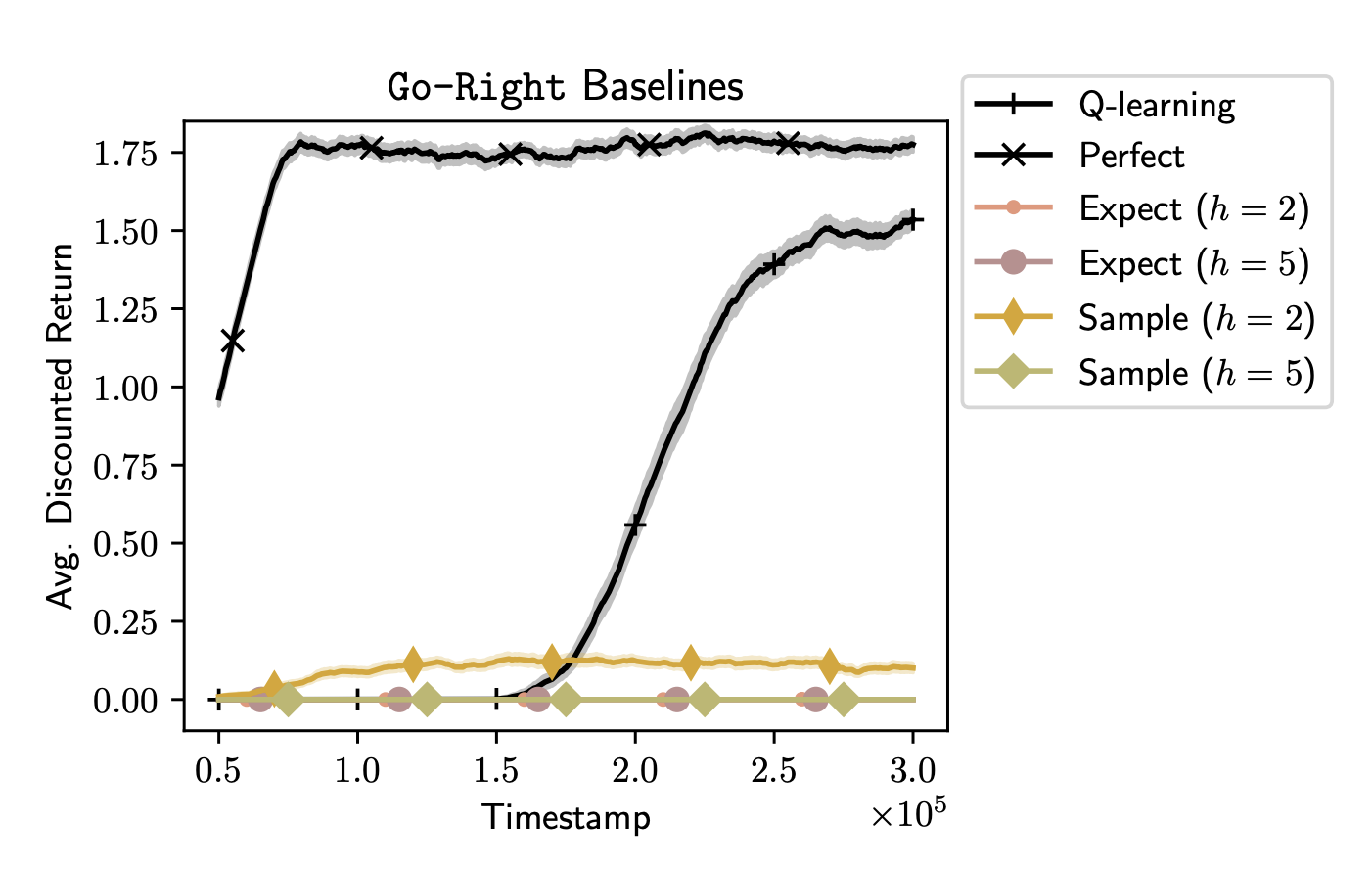
• Q-learning learns the optimal policy eventually but requires more steps, as it does not leverage any model-based planning.
• The Perfect Model shows that accurate predictions can drastically reduce the number of suboptimal actions, yielding higher returns.
• The Expectation Model may underpredict rare transitions (such as the full activation of prize indicators), leading to planning failures when the planning horizon is too long (e.g., $h=5$).
• Sampling Models capture stochasticity but often misrepresent rare events due to low-probability assignments.

Figure 3: Comparative performance of selective planning methods—Monte Carlo Target Variance (MCTV), Monte Carlo Target Range (MCTR), and Bounding-Box Inference (BBI)—in both the standard GoRight and the more challenging GoRight-10 (with 10 prize indicators) variants (Source: Talvitie et al., 2024).

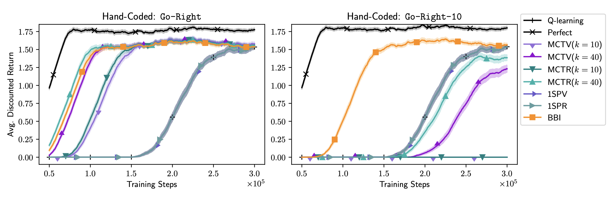
• Bounding-Box Inference (BBI):
  • In the GoRight-10 variant, BBI remains robust and largely insensitive to changes in the model’s predicted probability distribution.
  • However, when using learned models (especially neural networks), BBI can overestimate uncertainty due to cumulative looseness in bound propagation.

WIP

Results from learned models, discussions and conclusions will be included in a future update.

Feel free to reach out with any questions or comments. Happy experimenting!