Prediction and Control with Function Approximation

info

In this chapter, you'll learn about:

• Function Approximation in Reinforcement Learning: Using parameterized functions to estimate value functions in large or continuous state spaces.
• Feature Construction Techniques: Methods like coarse coding and tile coding to create features for linear function approximation.
• Gradient Descent and Semi-Gradient Methods: Techniques to optimize the parameters of value function approximations.
• Control with Function Approximation: Extending control methods like Sarsa, Expected Sarsa, and Q-Learning to work with function approximators for policy improvement.
• Average Reward Formulation: Introducing the average reward criterion as an alternative to discounted returns in continuing tasks.

In previous chapters, we explored tabular solution methods for reinforcement learning, including Dynamic Programming (DP), Monte Carlo (MC) methods, and Temporal-Difference (TD) learning. These methods allowed us to compute value functions and optimal policies by maintaining a table of values for each state or state-action pair. While effective for environments with small, discrete state spaces, tabular methods become impractical as the size or complexity of the state space increases. For example, a robot navigating using camera images cannot store a value for every possible image it might encounter.

To handle such scenarios, we introduce function approximation, where we use parameterized functions to estimate value functions. Function approximation allows us to generalize from seen states to unseen ones, enabling RL agents to operate in large or continuous state spaces.

This chapter explores prediction and control using function approximation. We will discuss various function approximators, including linear methods and neural networks, and how they can be applied to policy evaluation and control tasks.

Moving to Parameterized Functions

In tabular methods, we store a value for each state in a table. However, this approach doesn't scale to large or continuous state spaces. To overcome this limitation, we use parameterized functions that map states to value estimates. These functions are controlled by a set of weights or parameters that we adjust during learning.

For example, in a grid world, instead of storing a value for each position, we can use a function that computes the value based on the state's coordinates:

$$\hat{v}(s, \mathbf{w}) = w_1 x + w_2 y$$

Here, $x$ and $y$ are the coordinates of state $s$, and $w_1$ and $w_2$ are weights that we adjust during learning.

Linear Function Approximation

In linear function approximation, the value estimate is a linear combination of features:

$$\hat{v}(s, \mathbf{w}) = \mathbf{w}^\top \mathbf{x}(s)$$

• $\mathbf{x}(s)$ is the feature vector for state $s$.
• $\mathbf{w}$ is the weight vector.

The features $\mathbf{x}(s)$ are functions that extract relevant information from the state. The choice of features significantly impacts the approximation's quality.

Tabular Representation as a Special Case

Tabular value functions can be seen as a special case of linear function approximation. Each state $s$ has a unique feature vector $\mathbf{x}(s)$ where all elements are zero except for one element corresponding to state $s$, which is one. This is known as a one-hot encoding.

Non-Linear Function Approximation

Beyond linear functions, we can use non-linear function approximators like neural networks. Neural networks can capture complex patterns and relationships in the data, making them suitable for high-dimensional or continuous state spaces.

Feature Construction for Linear Methods

State Aggregation

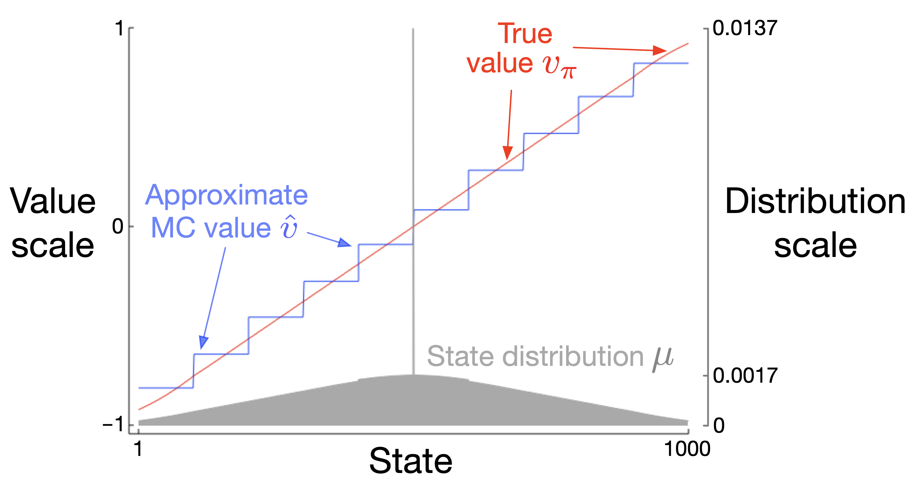
State aggregation groups similar states together and represents them with shared features. This reduces the number of parameters and introduces generalization across states within the same group.

Example

State aggregation in the 1000-state random walk problem, where the states are grouped into bins, yielding a stepwise approximation (blue) of the true value function (red). By aggregating states, the agent gains a coarser yet more compact representation, significantly reducing parameters while still capturing the broad trend of the value function. The figure is reproduced unaltered from the book.

Coarse Coding

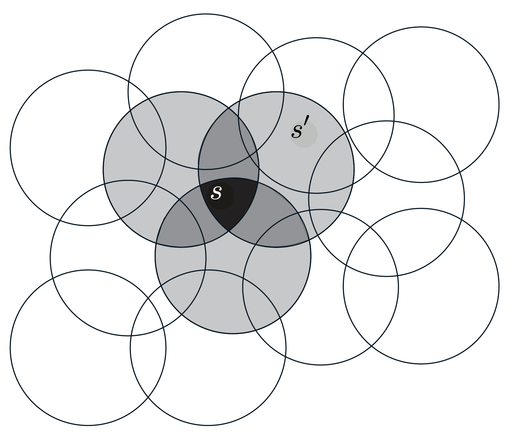
Coarse coding is a form of function approximation where features are activated over broad regions of the state space, often with overlapping receptive fields.

• Features: Each feature corresponds to a region in the state space.
• Activation: A feature is active if the current state falls within its receptive field.

Example

Coarse coding. The figure is reproduced unaltered from the book.

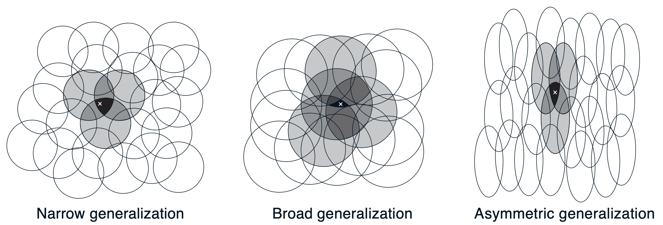
Coarse coding allows for both generalization (through overlapping features) and discrimination (by having multiple features with different receptive fields).

Example

Generalization in coarse coding. The figure is reproduced unaltered from the book.

Tile Coding

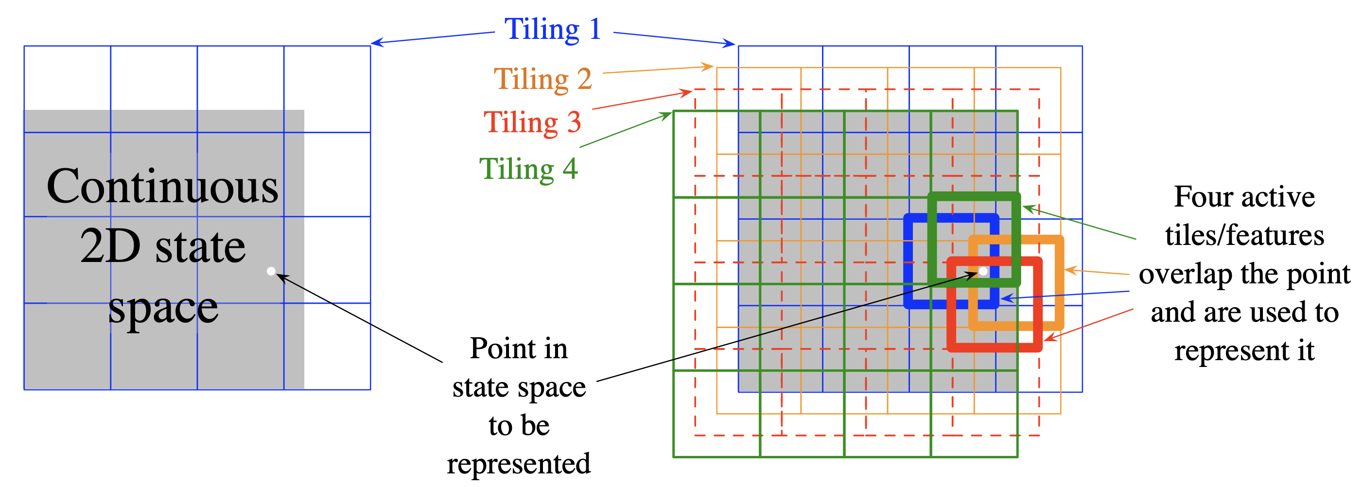
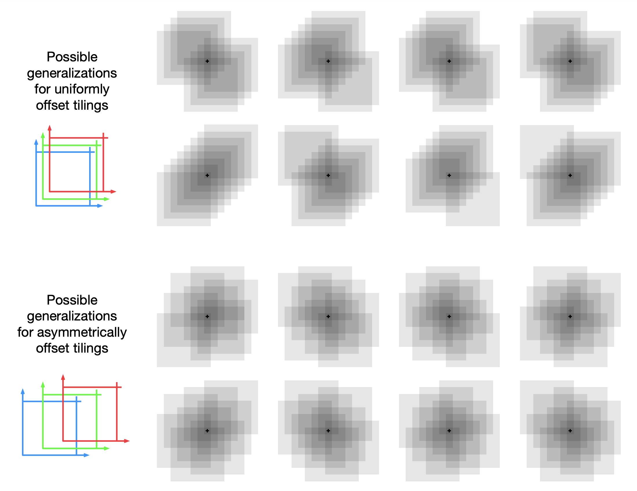
Tile coding is a computationally efficient form of coarse coding that uses multiple overlapping grids (tilings) to partition the state space.

• Tilings: Each tiling covers the state space with non-overlapping tiles.
• Offsets: Each tiling is slightly offset from others to create unique intersections.
• Features: A state activates one tile per tiling.

Tile coding provides a fixed, sparse representation that's efficient to compute and works well with linear function approximation.

Example

Tile coding. The figure is reproduced unaltered from the book.

Generalization

Generalization refers to the ability of the function approximator to apply knowledge learned from specific states to similar, unseen states. Generalization can speed up learning by reducing the amount of experience needed to learn accurate value estimates.

For example, a robot that learns to navigate in one room should be able to generalize that knowledge to navigate in similar rooms without starting from scratch.

Discrimination

Discrimination is the ability to distinguish between different states and assign them different value estimates. While generalization is beneficial, too much generalization can prevent the agent from accurately estimating the value of distinct states.

Ideally, we want a function approximator that provides both good generalization and good discrimination. However, there is often a trade-off between the two. The choice of features and the structure of the function approximator play crucial roles in achieving the right balance.

The shape, size, and overlap of receptive fields of coarse and tile coding affect generalization and discrimination:

• Larger Receptive Fields: More generalization but less discrimination.
• Smaller Receptive Fields: Less generalization but more discrimination.
• Overlap/offset: Allows for smoother generalization across states.

Example

Examples of generalization/discrimination with tile coding. The figure is reproduced unaltered from the book.

Recap

1. Why is function approximation necessary in reinforcement learning?

• It eliminates the need for policies.
• It allows RL to scale to large or continuous state spaces.
• It simplifies the reward function.
• It ensures faster convergence in all cases.

2. What is the primary difference between tabular methods and function approximation?

• Tabular methods are always more accurate than function approximation.
• Tabular methods require no memory, while function approximation does.
• Tabular methods store exact values, while function approximation generalizes using features.
• Function approximation can only be used with neural networks.

3. What is the main role of features in function approximation?

• To directly represent the reward function.
• To replace the policy in control tasks.
• To ensure exact solutions to the Bellman equation.
• To extract relevant information from the state for value estimation.

4. How does tile coding achieve generalization in function approximation?

• By using neural networks to calculate feature activations.
• By ensuring no overlap between features.
• By assigning each state to a single feature.
• By using multiple overlapping grids to activate features.

5. What is a key trade-off when choosing feature representations in function approximation?

• Learning rate vs. discount factor.
• Generalization vs. discrimination.
• On-policy vs. off-policy learning.
• Stability vs. exploration.

What's Next

The remainder of this chapter explores how function approximation methods are applied to both prediction (policy evaluation) and control (policy improvement) tasks:

1. On-policy Prediction
   Here, we focus on the case where the policy generating the data is the same as the policy being evaluated. We adapt Monte Carlo (MC) and Temporal-Difference (TD) ideas to function approximators and discuss how to handle features in high-dimensional or continuous state spaces.

2. On-policy Control
   We extend the concept of on-policy prediction to the control setting, where we use methods like semi-gradient Sarsa to optimize the policy while still using function approximation to represent action values.

3. Off-policy Methods
   Finally, we look at learning from a behavior policy different from the target policy, covering semi-gradient Q-learning, and Expected Sarsa with function approximation.