Convexity

info

In this chapter you'll be introduced to:

• Convex Sets: Understanding the definition of convex sets and identifying convex and non-convex sets.
• Convex Functions: Learning the formal definition of convex functions and how to determine if a function is convex.
• Equivalent Conditions for Convexity: Exploring first-order and second-order conditions that are equivalent to convexity.
• Optimality in Convex Functions: Understanding why any local minimum of a convex function is also a global minimum.
• Application to Linear Regression: Preparing to apply the concepts of convexity to the mean squared error loss function in linear regression.

In the previous chapter, we discussed the linear regression model, where we aimed to find the best-fitting line (or hyperplane) for our data by minimizing the mean squared error (MSE) loss function. To efficiently optimize the MSE loss and guarantee finding the global minimum, we need to understand the concept of convexity in functions and sets. Convexity plays a crucial role in optimization, particularly in machine learning algorithms.

Convex Sets

Definition

A set $X \subseteq \mathbb{R}^d$ is called convex if, for any two points $\mathbf{x}, \mathbf{y} \in X$ and any $\lambda$ where $0 \leq \lambda \leq 1$, the following condition holds:

$$\lambda \mathbf{x} + (1 - \lambda) \mathbf{y} \in X$$

This means that the line segment connecting any two points in the set is entirely contained within the set.

Examples

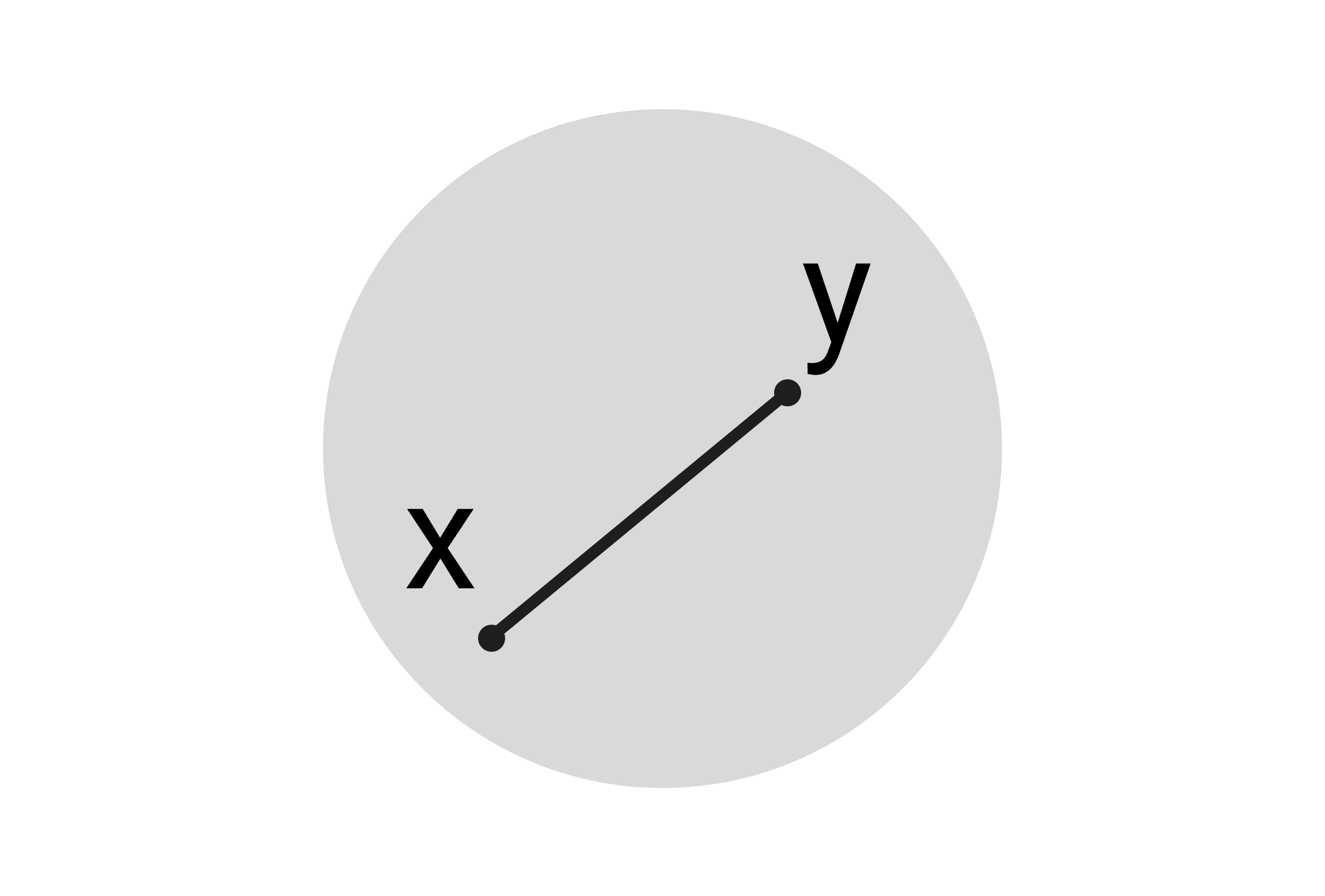
Convex Set

• Solid Circle (Disc): All points inside and on the boundary of a circle in $\mathbb{R}^2$ form a convex set.

• Polygon: Any convex polygon (e.g., square, triangle) is a convex set.

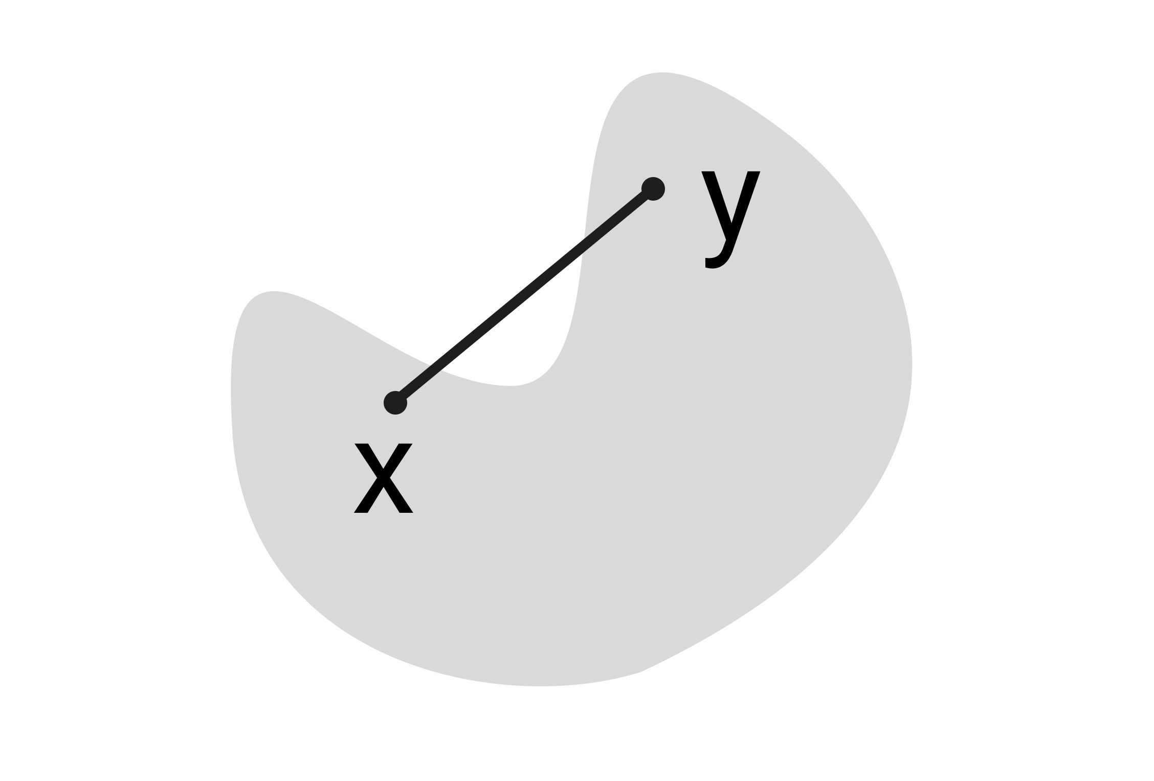
Non-Convex Set

• Shapes with Indentations: A shape like a crescent moon is not convex because some line segments between points in the set will pass outside the set.

• Disconnected Sets: If a set consists of two separate regions (e.g., two distinct circles), it's not convex because the line segment connecting a point from each region lies outside the set.

Convex Functions

Definition

A function $f: X \rightarrow \mathbb{R}$ is convex if:

1. The domain $X$ is a convex set.

2. For any $\mathbf{x}, \mathbf{y} \in X$ and any $\lambda$ where $0 \leq \lambda \leq 1$:

   $$f(\lambda \mathbf{x} + (1 - \lambda) \mathbf{y}) \leq \lambda f(\mathbf{x}) + (1 - \lambda) f(\mathbf{y})$$

This inequality implies that a straight line (or plane) between any two points on the function lies above the function itself.

Interpretation

• Curving Up: Convex functions curve upwards, and the line segment between any two points on the graph of the function lies above the graph.
• Affine Functions: Linear functions are considered convex because they satisfy the convexity condition with equality.

Examples

Convex Functions

1. Linear Functions:

   $$f(\mathbf{x}) = \mathbf{w}^\top \mathbf{x} + b$$
   • Any linear (affine) function is convex.
   • The convexity condition holds with equality.

2. Quadratic Functions:

   $$f(x) = x^2$$
   • The graph curves upwards.
   • Satisfies the convexity condition.

Non-Convex Functions

1. Concave Functions:

   $$f(x) = -x^2$$
   • The graph curves downwards.
   • Does not satisfy the convexity condition.

2. Functions with Discontinuities or Sharp Turns:

   • Functions that are not smooth or have points where the convexity condition fails.

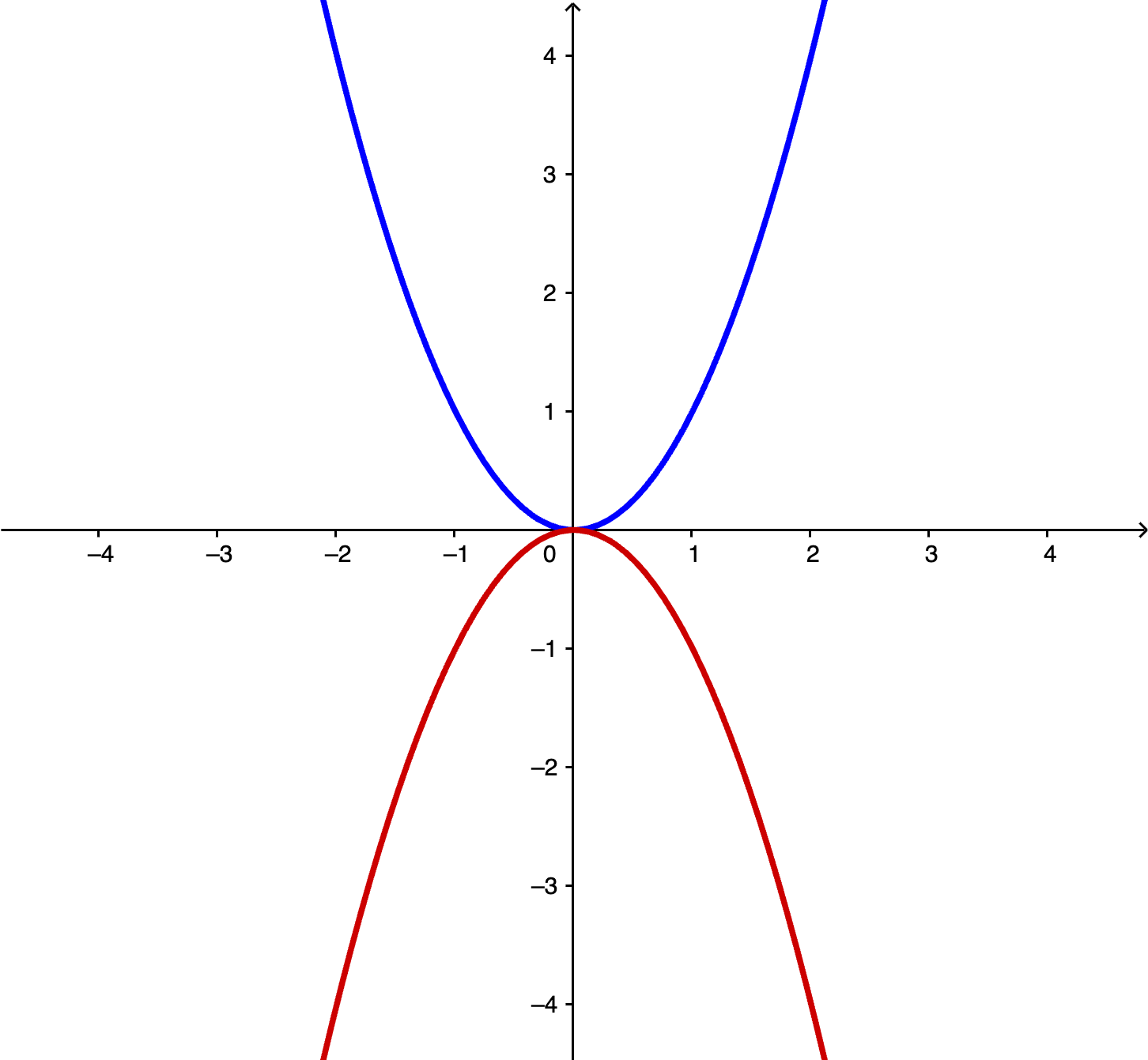
Examples:

• Blue Curve: Convex function (e.g., $f(x) = x^2$).
• Red Curve: Non-convex function (e.g., $f(x) = -x^2$).

Equivalent Conditions for Convexity

Determining whether a function is convex using the definition can be challenging. Fortunately, there are equivalent conditions that can simplify this process, especially for differentiable functions.

Theorem

Suppose $f: X \rightarrow \mathbb{R}$ is a twice-differentiable function on a convex set $X \subseteq \mathbb{R}^d$. The following statements are equivalent:

1. (Convexity): $f$ is convex.

2. (First-Order Condition): For all $\mathbf{x}, \mathbf{y} \in X$:

   $$f(\mathbf{y}) \geq f(\mathbf{x}) + \nabla f(\mathbf{x})^\top (\mathbf{y} - \mathbf{x})$$
   • Here, $\nabla f(\mathbf{x})$ is the gradient (vector of partial derivatives) of $f$ at $\mathbf{x}$.

3. (Second-Order Condition): For all $\mathbf{x} \in X$, the Hessian matrix $\nabla^2 f(\mathbf{x})$ is positive semidefinite.

   • A matrix is positive semidefinite if all its eigenvalues are non-negative.

Understanding the Conditions

First-Order Condition

• Geometric Interpretation: The function lies above its first-order Taylor expansion (tangent hyperplane) at any point $\mathbf{x}$.
• Implication: The tangent at any point is a global underestimator of the function.

Second-Order Condition

• Hessian Matrix: A square matrix of second-order partial derivatives.
• Positive Semidefinite: Indicates that the function curves upwards in all directions.

Proof Sketches

From First-Order to Convexity (B ⇒ A)

• Goal: Show that the first-order condition implies the convexity condition.
• Approach: Use the first-order condition to derive the convexity inequality by manipulating the expressions.

From Second-Order to First-Order (C ⇒ B)

• Goal: Show that if the Hessian is positive semidefinite, the first-order condition holds.
• Approach: Use Taylor's theorem to expand $f(\mathbf{y})$ around $\mathbf{x}$ and show that the remainder term is non-negative due to the positive semidefinite Hessian.

Optimality in Convex Functions

Global vs. Local Minima

• Global Minimum: A point $\mathbf{x}^*$ where $f(\mathbf{x}^*) \leq f(\mathbf{y})$ for all $\mathbf{y} \in X$.
• Local Minimum: A point $\mathbf{x}^*$ where $f(\mathbf{x}^*) \leq f(\mathbf{y})$ for all $\mathbf{y}$ in some neighborhood around $\mathbf{x}^*$.

Theorem

For a convex function $f: X \rightarrow \mathbb{R}$:

• Any local minimum is also a global minimum.

Implications

• Optimization Simplification: When optimizing convex functions, finding a local minimum suffices.
• Guarantees in Optimization Algorithms: Algorithms that converge to a local minimum will also find the global minimum for convex functions.

Proof Outline

• Assumption: Suppose $\mathbf{x}^*$ is a local minimum.
• Goal: Show that $f(\mathbf{x}^*) \leq f(\mathbf{y})$ for all $\mathbf{y} \in X$.
• Approach:
  • Use the convexity condition to establish an inequality between $f(\mathbf{x}^*)$ and $f(\mathbf{y})$.
  • Show that any deviation from $\mathbf{x}^*$ cannot result in a lower function value.

Application to Linear Regression

Understanding convexity is essential for optimizing the mean squared error (MSE) loss function in linear regression.

Mean Squared Error Loss Function

Given:

• Hypothesis Class:

  $$h(\mathbf{x}) = \mathbf{w}^\top \mathbf{x}$$

• Training Data:

  $$\{ (\mathbf{x}^{(m)}, t^{(m)}) \}_{m=1}^M$$

• MSE Loss:

  $$J(\mathbf{w}) = \frac{1}{2M} \sum_{m=1}^M \left( h(\mathbf{x}^{(m)}) - t^{(m)} \right)^2$$

Convexity of MSE Loss

• Objective: Show that $J(\mathbf{w})$ is a convex function of $\mathbf{w}$.
• Importance:
  • Ensures that any local minimum of $J(\mathbf{w})$ is also a global minimum.
  • Simplifies the optimization process for finding the best parameters $\mathbf{w}$.

Next Steps

In the next chapter, we'll:

• Prove the convexity of the MSE loss function.
• Explore optimization techniques for finding the optimal weights $\mathbf{w}$.
• Discuss properties of convex optimization problems.

Recap

In this chapter, we've covered:

• Convex Sets: Defined convex sets and identified examples.
• Convex Functions: Provided the formal definition and examples of convex and non-convex functions.
• Equivalent Conditions: Introduced first-order and second-order conditions equivalent to convexity.
• Optimality: Demonstrated that any local minimum of a convex function is also a global minimum.
• Relevance to Linear Regression: Prepared to apply these concepts to optimize the MSE loss function.