Training Data

The quality and quantity of training data are critical to the success of any machine learning project. Effective sampling, labeling, handling class imbalance, and data augmentation are essential techniques to prepare robust datasets that improve model performance and generalization. This chapter explores various methods for creating and refining training datasets, ensuring they are comprehensive, representative, and suitable for training accurate and reliable machine learning models.

Sampling

Sampling occurs at several stages of an ML project lifecycle (e.g., sampling real-world data to create training data; sampling from a dataset to create training/validation/test splits; sampling events for better monitoring the ML system, etc.) and is often overlooked in typical ML coursework. Choosing the right sampling method helps mitigate possible biases and improves data efficiency.

Nonprobability Sampling

Nonprobability sampling is not based on any probability criteria. The samples selected are not representative and are often riddled with selection bias. Common methods include:

• Convenience sampling: Samples of data are selected based on their availability.
• Snowball sampling: Future samples are selected based on existing samples. For example, when scraping legitimate Twitter accounts, you start with a small number of accounts, then you scrape all accounts they follow.
• Judgment sampling: Experts decide which samples to include.
• Quota sampling: Samples are selected based on quotas for slices of data without randomization or knowledge of the underlying distribution.

Examples of applications that use this kind of sampling include large language models (text available on Wikipedia, Common Crawl, and Reddit); sentiment analysis (data collected from IMDB reviews or Amazon, which are biased toward users who leave reviews online); and self-driving cars (initially with data only available in areas where regulation permitted, e.g., Phoenix, Arizona, and the Bay Area).

Simple Random Sampling

Simple random sampling draws samples uniformly, regardless of the data distribution. Models trained with data sampled in this way might think rare classes don't exist due to the lack of representatives in the training data.

Stratified Sampling

This method splits data into groups we care about (e.g., groups related to the classes/labels or a specific feature) and then samples data from these groups. This ensures representation of each group in the training data. The drawback is that in some cases, this is not possible, such as in multi-label tasks.

Weighted Sampling

In weighted sampling, we assign each sample a probability of being selected. This allows us to leverage domain expertise to change a model's decision boundary. We can assign more weight to more relevant samples (e.g., more recent samples) or to mimic the distribution of the real world that is not represented in the collected data.

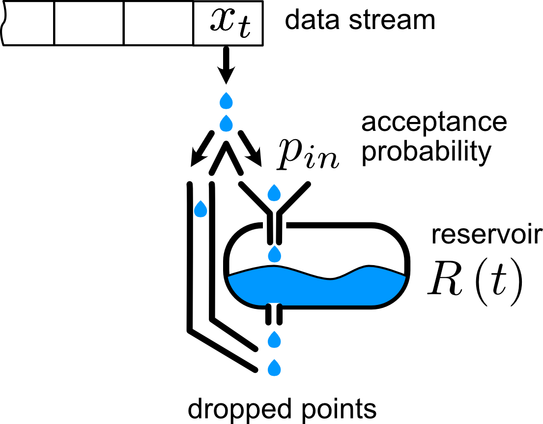
Reservoir Sampling

Reservoir sampling is a technique used when dealing with streaming data or when the total number of data points is unknown. It allows for maintaining a random sample of a fixed size from a potentially large or infinite stream of data. This is particularly useful when it's impractical to store the entire dataset in memory. The algorithm is:

1. Initialize a reservoir of size $k$;
2. Fill the reservoir with the first $k$ data points;
3. For each subsequent data point, the $n^{\text{th}}$ data point (where $n > k$), generate a random number $i \in [1, n]$, and replace the $i^\text{th}$ element of the reservoir if $i \le k$.

This ensures that each data point has an equal probability, $k/n$, of being included in the sample.

Importance Sampling

Importance sampling is a statistical technique used to estimate properties of a target distribution by sampling from a different distribution. This method is particularly useful in situations where it is difficult to sample directly from the target distribution, but easier to sample from an auxiliary distribution. So, if we have a distribution P(x) that is really expensive, slow, or unfeasible to sample from, we can define a proposal distribution or importance distribution $Q(x)$ that we can sample and weight this sample by $P(x)/Q(x)$. The following equation shows that, in expectation, $x$ sampled from $P(x)$ is equal to $x$ sampled from $Q(x)$ weighted by $P(x)/Q(x)$:

$$\mathbb{E}_{P(x)}[x] = \sum_x P(x)x = \sum_x Q(x)x\frac{P(x)}{Q(x)} = \mathbb{E}_{Q(x)} \bigg[ x\frac{P(x)}{Q(x)} \bigg]$$

Importance sampling is highly applicable in reinforcement learning, specially in off-policy algorithms, where the agent's behavior and target policies differ. That is, the agent learns from data collected by a different policy that the one it is currently trying to optimize. Importance sampling allows us to correct the bias by weighting the returns according to the probability of actions under the new policy, and then reuse historical data.

Labeling

Labeling is a core component of any supervised ML system. The performance of an ML model depends heavily on the quantity and quality of the labeled data it's trained on.

Hand Labels

Hand-labeling data can be expensive, especially if the data requires subject matter expertise (SME). For instance, labeling chest X-rays would require board-certified radiologists, whose time is limited and costly. Additionally, data privacy concerns must be addressed.

Manual labeling is also a very slow process. For example, to achieve an accurate transcription of speech utterance at the phonetic level, it is estimated to take 400 times longer than the duration of the utterance. This can make the system less adaptive to changing environments and requirements.

Label Multiplicity

When different sources or annotators provide data, it's common to have conflicting labels for a data instance, especially if the level of expertise required is high. Establishing ground rules and providing training to align labelers is essential.

Data Lineage

The system must be capable of differentiating data from multiple sources and labeling techniques using data lineage. This helps flag potential biases in the data and debug the models effectively.

Natural Labels

Some tasks have natural ground truth labels, such as stock prediction or recommendation systems. Even if a task doesn't have natural labels, it can often be reframed to generate feedback on the predictions. For instance, offering users the option to submit a different translation in a translation system or using a like button in a newsfeed ranking task are forms of generating new labels.

Feedback Loop Length

Choosing the appropriate length for the feedback loop requires careful consideration and depends heavily on the task. It's a trade-off between speed and accuracy. For instance, a recommendation system on Amazon might receive feedback within minutes, while systems dealing with longer content, such as YouTube videos or blog posts, might have longer feedback loops. A short window allows for quicker detection of issues and faster adjustments, but it may also lead to premature labeling of recommendations before receiving complete feedback.

Feedback can come in different formats and at various stages of the system. For example, in an e-commerce application, feedback could include clicking on a product, adding a product to the cart, purchasing a product, rating, leaving a review, or returning a previously bought product.

Handling the Lack of Labels

Method	How	Ground truths required?
Weak Supervision	Leverages (often noisy) heuristics to generate labels.	No, but a small number of labels are recommended to guide the development of heuristics.
Semi-Supervision	Leverages structural assumptions to generate labels.	Yes, a small number of initial labels as seeds to generate more labels.
Transfer Learning	Leverages models pretrained on another task for your new task.	No for zero-shot learning. Yes for fine-tuning, though the number of ground truths required is often much smaller than what would be needed if you train the model from scratch.
Active Learning	Labels data samples that are most useful to your model.	Yes.

Weak Supervision

One of the most popular tools for weak supervision is Snorkel, developed by the Stanford AI Lab. This tool relies on the concept of labeling functions (LFs), which encode heuristics. These heuristics can be based on keywords, regular expressions, database lookups, the outputs of other models, etc.

Semi-supervision

Several semi-supervised techniques have been developed over the years. One of them is self-training, where you start by training a model on your existing set of labeled data and use this model to make predictions for unlabeled samples. You can expand your training set with high-probability labels and continue this process until you're satisfied with the results.

Additionally, clustering algorithms can label samples based on similarity with labeled samples. Another method is the perturbation-based approach, where you add perturbations to labeled samples to generate new samples with the same label, assuming the perturbations don't change the labels. This method is further discussed in the data augmentation section.

Transfer Learning

In transfer learning, a base model is trained on a base task with abundant training data (e.g., language modeling with next-token prediction). This model can then be used in a zero-shot scenario or fine-tuned for a downstream task. Fine-tuning involves tweaking the base model, such as continuing its training on data from the target task.

Active Learning

Active learning involves labeling data samples that are most useful to the model, based on specific metrics or heuristics. The most straightforward metric is uncertainty measurement, where you label the examples the model is least certain about, hoping they will help the model learn the decision boundary better. Another method is query-by-committee, which is based on the disagreement among an ensemble of candidate models.

Recommended Readings

For a more comprehensive review of active learning methods, it's recommended to read Burr Settles's paper Active Learning Literature Survey

Class Imbalance

Class imbalance is a common issue in many machine learning problems, where certain classes are significantly underrepresented compared to others. This can lead to models that perform well on the majority class but poorly on the minority class, resulting in biased and ineffective predictions. And in some applications, you're interested on the performance on the rare cases (i.e., detecting lung cancer).

Challenges of Class Imbalance

1. Biased Predictions: The model tends to be biased towards the majority class, often ignoring the minority class, leading to poor performance on the latter. In the extreme case where there is no instance of the rare class in the training set, the model might assume these rare classes don't exist.
2. Skewed Metrics and Overfitting: The model might overfit to the majority class, failing to generalize well to the minority class or unseen data. It's easier for the model get stuck in a nonoptimal solution by exploiting simple heuristics, for example, if the model learns to always outputs the majority class and its accuracy is already 99%.
3. Asymmetric Costs of Error: The cost of a wrong prediction on a sample of the rare class might be much higher than a wrong prediction on a sample of the majority class, such as in the lung cancer detection example. Misclassification on an X-ray with cancerous cells is much more dangerous than misclassification on an X-ray of a normal lung.

Handling Class Imbalance

Addressing class imbalance involves various techniques at both the data and algorithm levels to ensure that the model can learn effectively from imbalanced data.

Recommended Readings

For a more comprehensive review of class imbalance methods, it's recommended to read Johnson and Khoshgoftaar's paper Survey on deep learning with class imbalance

Using the Right Evaluation Metrics

Instead of relying on accuracy, use evaluation metrics that provide a clearer picture of the model's performance on imbalanced data:

• Precision and Recall: Measure the accuracy of positive predictions and the ability to find all positive instances.
• F1 Score: The harmonic mean of precision and recall, providing a single metric that balances both.

F1, precision, and recall are asymmetric metrics, which means that their values change depending on which class is considered the positive class.

• Area Under the ROC Curve (AUC-ROC): Evaluates the trade-off between true positive and false positive rates.

• Area Under the Precision-Recall Curve (AUC-PR): Particularly useful for imbalanced datasets, focusing on the performance for the minority class.

Data-Level Methods: Resampling

Data-level methods modify the distribution of the training data to reduce imbalance. There are two primary techniques: undersampling the majority class and oversampling the minority class.

• Undersampling: This involves reducing the number of samples in the majority class. The simplest method is to randomly remove samples. Another technique is Tomek links, where samples from the majority class that are close to minority class samples are removed, helping to clarify the decision boundary. However, this can make the model less robust to subtle differences between classes.

• Oversampling: This involves increasing the number of samples in the minority class. The simplest method is to randomly duplicate existing samples. A more sophisticated technique is SMOTE (Synthetic Minority Oversampling Technique), which generates new minority class samples by interpolating between existing samples. SMOTE works well with low-dimensional data but can introduce noise if overused.

Both Tomek links and SMOTE, along with other techniques like Near-Miss and one-sided selection, are effective for low-dimensional data.

Avoiding Overfitting

Overfitting is a risk when using resampling techniques. Oversampling can lead to overfitting on the resampled training data, while undersampling can result in the loss of valuable information. To mitigate these risks, consider the following strategies:

• Two-Phase Learning: Train the model initially on the resampled data, then fine-tune it on the original data. This helps the model generalize better.
• Dynamic Sampling: Adjust the sampling strategy dynamically during training. For example, oversample low-performing classes and undersample high-performing classes to balance the learning process. This method helps the model focus on areas it hasn't learned well yet.

Algorithm-Level Methods

Algorithm-level methods keep the data distribution intact but alter the learning algorithm to make it more robust to imbalance. These methods often adjust the weights for samples in the loss function, emphasizing the learning of minority class instances.

• Cost-sensitive learning: Define a cost matrix to specify the cost of each possible outcome of the model concerning the correct label. For example:

	Actual Negative	Actual Positive
Predicted Negative	$C_{00}$	$C_{10}$
Predicted Positive	$C_{01}$	$C_{11}$

We then have the loss function:

$$\mathcal{L}(x;\theta) = \sum_j C_{ij} \, P(j|x;\theta)$$

• Class-balanced loss: This method modifies the loss function to weigh the contributions of each class based on their prevalence in the dataset. This ensures that the minority class has more influence on the loss. A more advanced version of this method accounts for the overlap among existing samples, such as the class-balanced loss based on the effective number of samples:

$$\begin{gather*} W_i = \frac{N}{\text{number of samples of class i}}, \qquad \text{where N is the total number of training samples} \\ \\ \mathcal{L}_{\text{weighted}}(x;\theta) = W_i \sum_j P(j|x;\theta) \, \mathcal{L}(x,j) \end{gather*}$$

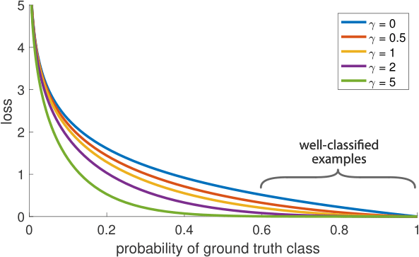
• Focal loss: Focal loss increases the weight for instances that are harder for the model to classify (i.e., those with lower prediction probabilities). The formula for focal loss, compared to cross-entropy, is:

$$\begin{gather*} CE(\rho_t) = - \log(\rho_t) \\ FL(\rho_t) = - (1-\rho_t)^\gamma \log(\rho_t) \end{gather*}$$

Data Augmentation

Data augmentation is a technique used to artificially increase the size and diversity of a training dataset without collecting new data. Data augmentation is particularly useful in scenarios where data collection is expensive or time-consuming. However, even when data is abundant, augmented data can make our models more robust to noise and even adversarial attacks.

Simple Label-Preserving Transformations

Simple label-preserving transformations involve applying basic modifications to the existing data that do not alter the underlying class label. These transformations are particularly useful for image and text data.

Image Data

• Rotation: Rotating images by a certain degree (e.g., 90°, 180°, 270°).
• Translation: Shifting images horizontally or vertically.
• Scaling: Resizing images.
• Flipping: Mirroring images horizontally or vertically.
• Color Jittering: Randomly changing the brightness, contrast, saturation, and hue.
• Cropping: Randomly cropping and resizing images back to the original size.

Text Data

• Synonym Replacement: Replacing words with their synonyms.
• Random Insertion: Inserting random words into the text.
• Random Deletion: Deleting random words from the text.
• Shuffling: Shuffling the order of words or phrases in the text.

Perturbation

Perturbation-based augmentation involves adding small, controlled changes to the data that preserve the original label. These changes are usually subtle and designed to simulate natural variations in the data or even be make to fool a neural network. Su at al. showed that 67.97% of the natural images in the Kaggle CIFAR-10 test dataset and 16.04% of the ImageNet test images can be misclassified by changing just one pixel.

Perturbation can be injected by adding noise, either random noise or by search strategy (i.e., DeepFool). One of the most notable examples is BERT, where the model chooses 15% of all tokens in each sequence at random and chooses to replace 10% of the chosen tokens with random words.

Recommended Readings

• Goodfellow et al., Explaining and Harnessing Adversarial Examples.
• Moosavi-Dezfooli et al., DeepFool: a simple and accurate method to fool deep neural networks.
• Miyato et al., Virtual Adversarial Training: A Regularization Method for Supervised and Semi-Supervised Learning

Data Synthesis

Data synthesis involves generating entirely new data points based on the distribution of the existing dataset. This technique can be particularly useful when dealing with rare classes or when collecting new data is impractical.

• Generative Adversarial Networks (GANs): GANs can generate new data points by training a generator network to produce realistic samples that can fool a discriminator network. This method is widely used for image synthesis but can also be applied to other data types.

• Mixup: Combining two data points to create a new one by taking a weighted average of their features and labels. This encourages the model to learn more linear decision boundaries.

  Example of Mixup:

  $$\begin{gather*} \tilde{x} = \lambda x_i + (1 - \lambda) x_j \\ \tilde{y} = \lambda y_i + (1 - \lambda) y_j \end{gather*}$$

  Where $x_i, x_j$ are input data points, $y_i, y_j$ are their labels, and $\lambda$ is a random value between 0 and 1.

Recommended Readings

refs="https://arxiv.org/abs/1710.09412||Zang et al., mixup: Beyond Empirical Risk Minimization;;; https://www.nature.com/articles/s41598-019-52737-x||Sandfort et al., Data augmentation using generative adversarial networks (CycleGAN) to improve generalizability in CT segmentation tasks;;; https://journalofbigdata.springeropen.com/articles/10.1186/s40537-019-0197-0||Shorten et al., A survey on Image Data Augmentation for Deep Learning" %}