Model Development and Offline Evaluation

Six Tips for Model Selection

1. Avoid the state-of-the-art trap: Don’t be swayed by the latest and most complex algorithms just because they are state-of-the-art. Often, simpler models can perform just as well or better, especially if they are well-tuned and well-understood. Remember that researchers often evaluate models in academic settings, which we discussed in Chapter 1.

2. Start with the simplest models: Begin with simple models like linear regression or decision trees. These models are easier to interpret and debug. Once you establish a baseline performance and ensure your training and prediction pipelines are consistent, you can move to more complex models if necessary. While you can start with more complex models that require little effort to get started (e.g., a pretrained version of BERT from Hugging Face's Transformers), always test simpler models to verify that the more complex solution indeed outperforms them.

   Simple is better than complex

3. Avoid human biases in selecting models: Ensure that model selection is based on objective performance metrics rather than subjective preferences or biases. If an engineer is more enthusiastic about a specific solution, they may spend more time tuning it. Make sure to compare architectures under similar setups.

4. Evaluate good performance now versus good performance later: Consider both short-term and long-term performance. Some models might perform well initially but degrade over time, while others might improve as more data is collected. Regularly monitor model performance and be prepared to update or replace models as necessary.

5. Evaluate trade-offs: Every model comes with trade-offs. Consider factors such as training time, inference time, scalability, interpretability, and resource requirements, as well as the trade-off between false positives and false negatives. Choose a model that balances these factors in a way that aligns with your project goals.

6. Understand your model's assumptions: Each model makes specific assumptions about the data. Ensure that these assumptions hold for your dataset. For example:

   1. Prediction assumption: It's possible to predict $Y$ based on $X$.
   2. IID: Neural Networks assume that examples are independent and identically distributed.
   3. Smoothness: If an input $X$ produces an output $Y$, then an input close to $X$ would produce an output proportionally close to $Y$.
   4. Tractability: Let $X$ be the input and $Z$ be the latent representation of $X$. Every generative model makes the assumption that it's tractable to compute the probability $\mathbb{P}(Z\|X)$.
   5. Boundaries: A linear classifier assumes that decision boundaries are linear.
   6. Conditional independence: A naive Bayes classifier assumes that the attribute values are independent of each other given the class.
   7. Normally distributed: Many statistical methods assume that data is normally distributed.

Ensembles

Ensemble methods combine multiple models to improve overall performance, robustness, and generalization capabilities. By leveraging the strengths of different models, ensemble techniques can often achieve better results than individual models (base learners). The effectiveness of an ensemble depends on the diversity and independence of the individual models: the less correlated the models, the better the ensemble performance. Thus, creating an ensemble with different architectures of models can significantly boost performance.

Although ensemble methods can provide substantial performance improvements, they are less favored in production due to their complexity in deployment and maintenance. However, they remain common in scenarios where even a small performance boost can lead to significant financial gains, such as predicting click-through rates for advertisements.

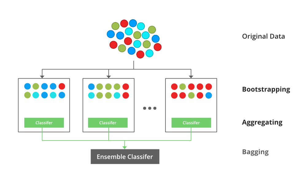
Bagging

Bagging, or Bootstrap Aggregating, aims to reduce variance and prevent overfitting by training multiple instances of the same model on different subsets of the training data. These subsets are generated by random sampling with replacement (bootstrap sampling). The predictions of these models are then aggregated, typically by averaging for regression tasks or majority voting for classification tasks.

Random Forests are a popular implementation of bagging, where multiple decision trees are trained on different subsets of the data and their predictions are averaged or voted upon to produce the final output. Random Forests also introduce additional randomness by selecting a random subset of features at each split in the trees, further reducing correlation among trees.

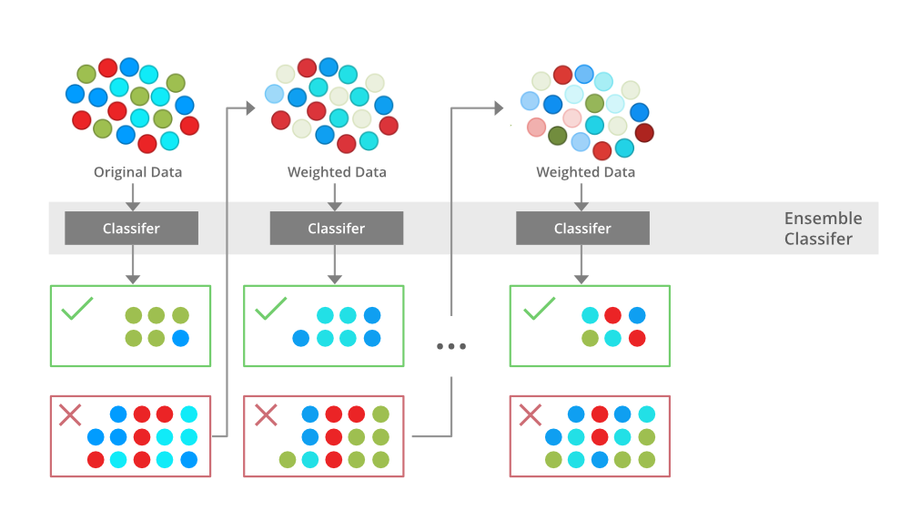
Boosting

Boosting aims to reduce bias and improve model accuracy by sequentially training models, where each new model attempts to correct the errors made by the previous models. This process focuses more on difficult instances that were misclassified or had higher errors in previous iterations. The final prediction is typically a weighted sum of the predictions from all models.

AdaBoost, short for Adaptive Boosting, assigns weights to each training instance and adjusts them after each iteration. Misclassified instances receive higher weights, forcing the next model to focus more on those hard-to-classify cases. The final model is a weighted sum of the individual models' predictions.

Gradient Boosting builds models sequentially, with each new model being trained to predict the residuals (errors) of the previous models. By minimizing these residuals, Gradient Boosting effectively improves the model's accuracy over iterations. Gradient Boosting Machines (GBMs), such as XGBoost, LightGBM, and CatBoost, are popular implementations that offer efficient training and strong performance.

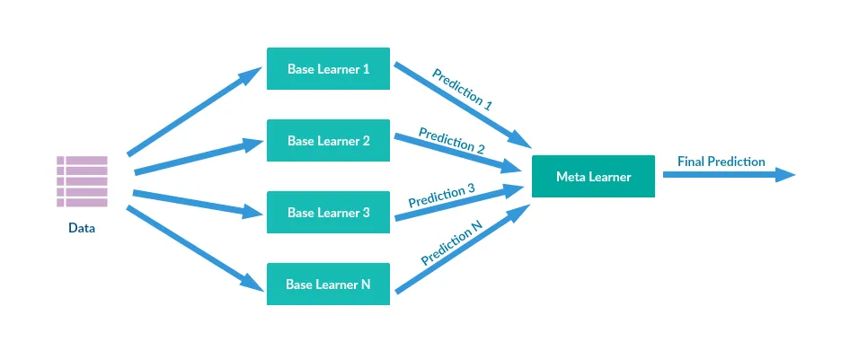
Stacking

Stacking, or Stacked Generalization, involves training multiple base models and then using their predictions as inputs to a higher-level meta-model. The meta-model learns to combine the predictions and make the final predictions. The meta-model can be either a heuristic or another model. This approach allows for leveraging different types of models and their unique strengths.

Experiment Tracking and Versioning

Experiment tracking and versioning are practices in machine learning to ensure reproducibility, facilitate debugging, and manage the iterative nature of model development. By systematically tracking experiments you can compare different setups (architecture, hyperparameters, initialization, etc.) and better understand how changes affect your model's performance.

Experiment Tracking

Experiment tracking involves recording all aspects of an experiment, including configurations, code, data, results, and metrics. This helps in comparing different experiments, understanding what changes lead to performance improvements, and ensuring reproducibility. A short list of things you might want to consider tracking for each experiment during its training:

• The configuration for the experiment, such as: hyperparameters, model architecture, data preprocessing steps, and other configuration settings.
• The loss curve corresponding to the train split and each of the eval splits.
• The model performance metrics such as accuracy, loss, precision, recall, F1 score, and any custom metrics relevant to the project.
• The log of corresponding sample, prediction, and ground truth label. This comes in handy for ad hoc analytics and sanity checks.
• The speed of your model, evaluated by the number of steps per second or, if your data is text, the number of tokens processed per second.
• System performance metrics such as memory usage and CPU/GPU utilization. They're important to identify bottlenecks and avoid wasting system resources.

Versioning

Versioning ensures that different versions of datasets, code, and models are systematically managed and can be reproduced or reverted to as needed.

Debugging ML Models

Recommended Readings

For more comprehensive understanding of the topic, it's recommended Andrej Karpathy's blog post A Recipe for Training Neural Networks

Some steps and strategies for debugging ML models according to Karpathy's blog:

1. Become One with the Data

   • Spend significant time understanding and visualizing the data.
   • Look for patterns, imbalances, biases, and outliers.
   • Write code to filter, sort, and visualize data distributions and outliers.

2. Set Up End-to-End Training and Evaluation Skeleton

   • Start with a simple model (e.g., a linear classifier) to set up the training and evaluation pipeline.
   • Fix random seeds to ensure reproducibility.
   • Disable unnecessary features like data augmentation initially.
   • Verify that the initial loss and model behavior are as expected.
   • Use human-interpretable metrics and baselines for comparison.
   • Overfit a single batch to verify the model can learn properly.

3. Overfit

   • Initially, focus on overfitting a large model to the training data to ensure it can achieve a low error rate.
   • Choose a well-established model architecture related to your problem.
   • Use a forgiving optimizer like Adam with an appropriate learning rate.
   • Gradually introduce complexity and verify performance improvements.

4. Regularize

   • Once the model overfits, introduce regularization to improve validation accuracy.
   • Add more data if possible, as it is the best way to regularize.
   • Use data augmentation and pretrained models.
   • Reduce input dimensionality and model size if appropriate.
   • Apply techniques like dropout, weight decay, and early stopping.

5. Tune

   • Explore a wide range of hyperparameters using random search rather than grid search.
   • Consider hyperparameter optimization tools for more systematic tuning.

6. Squeeze Out the Juice

   • Once the best model and hyperparameters are found, use ensembles to boost performance.
   • Let models train longer than initially expected, as they often continue to improve.

Distributed Training

As models are getting bigger and more resource-intensive, companies care a lot more about training at scale. It's common to train a model using data that doesn't fit into memory. In these cases, our algorithms for preprocessing, shuffling, and batching data will need to run out-of-core and in parallel.

In some cases, a single data sample is so large it can't fit into memory, and we'll have to use something like gradient checkpointing. Even when a sample fits into memory, using checkpointing can allow you to fit more samples into a batch, which might allow you to train your model faster.

Data Parallelism

Data parallelism involves splitting the dataset into smaller chunks and distributing them across multiple devices (e.g., GPUs or nodes). Each device trains a copy of the model on its subset of the data, and you accumulate the gradients across devices to update the model parameters.

Synchronous Stochastic Gradient Descent (SGD)

In synchronous SGD, all devices wait until every device has completed its gradient computation for the current batch before averaging the gradients and updating the model parameters. This ensures that each device is working with the same model parameters at each step, leading to more stable convergence.

Asynchronous Stochastic Gradient Descent (SGD)

In asynchronous SGD, devices do not wait for each other to complete their gradient computations. Instead, each device independently updates the model parameters as soon as it finishes its computations. This approach can lead to faster training times as devices are not idly waiting, but it can introduce inconsistencies in the model parameters across devices, potentially affecting convergence stability.

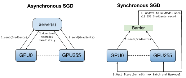
Asynchronous SGD theoretically converges with more steps than synchronous SGD. However, in practice, with a large number of weights, gradient updates are typically sparse, affecting only small fractions of the parameters. This reduces conflicts between updates from different machines. Consequently, gradient staleness is minimized, and the model converges similarly for both synchronous and asynchronous SGD.

Model Parallelism

Model parallelism involves splitting the model itself across multiple devices. Different parts of the model are assigned to different devices, and the forward and backward passes are executed across these devices. This approach is useful when the model is too large to fit into the memory of a single device.

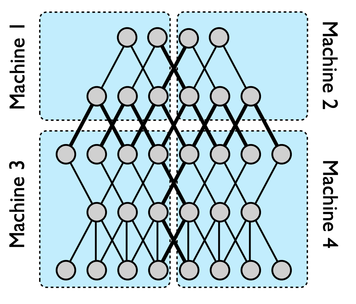
Pipeline parallelism involves splitting the model into stages and distributing these stages across multiple devices. Each device processes a different part of the model, passing intermediate results to the next device in the pipeline.

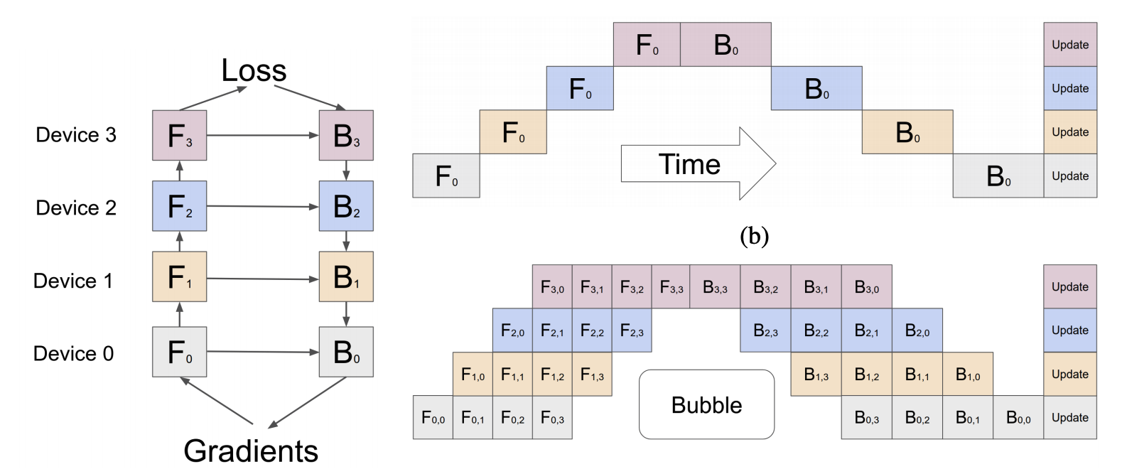
In practice, combining both data parallelism and model parallelism can be beneficial, especially for very large models and datasets.

AutoML

Automated Machine Learning (AutoML) encompasses techniques and tools designed to automate parts of the machine learning pipeline. AutoML can significantly reduce the time and expertise required to build high-performing models by automating tasks such as hyperparameter tuning, feature selection, and model selection. AutoML can be broadly categorized into Soft AutoML and Hard AutoML.

Soft AutoML: Hyperparameter tuning

Hyperparameter tuning involves finding the best set of hyperparameters that maximize model performance. Soft AutoML focuses on automating this process to enhance efficiency and performance.

Key Techniques in Hyperparameter Tuning:

• Grid Search: Exhaustively searches over a specified parameter grid to find the optimal hyperparameters. While thorough, it can be computationally expensive.
• Random Search: Randomly samples hyperparameter combinations within a specified range. It is more efficient than grid search and can often find good hyperparameters with fewer iterations.
• Bayesian Optimization: Uses a probabilistic model to predict the performance of hyperparameter combinations and iteratively improves this model to find the optimal set. This method balances exploration and exploitation, making it more efficient than random search.
• Hyperband: Combines random search with an early stopping strategy to allocate resources to promising hyperparameter configurations while discarding poor performers early.

Danger

Never use your test split to tune hyperparameters. Choose the best set of hyperparameters for a model basedon a validation split, then report the model's final performance on a test split.

Hard AutoML: Architecture search and learned optimizer

Hard AutoML involves more complex tasks, such as neural architecture search (NAS) and the development of learned optimizers, to automate the design and training of machine learning models.

A NAS setup consists of three components:

1. A Search Space: Defines possible model architectures, the building block to choose from and constraints on how they can be combined.
2. A Performance Estimation Strategy: To evaluate the performance of a candidate architecture without having to train each candidate architecture from scratch until convergence.
3. A Search Strategy: Some common approaches are random search, reinforcement learning (rewarding the choices that improve performance estimation) and evolution (adding mutations to an architecture, choosing the best-performing ones, and so on).

Learned optimizers are trained on various tasks to develop effective optimization strategies that generalize across different problems. The creation process involves training a meta-optimizer on a diverse set of tasks, this meta-optimizer can then be applied to new tasks, improving convergence rates and overall model performance. The beauty of this approach is that this learned optimizer can then be used to train a better-learned optimizer.

Model Offline Evaluation

Work in Progress

Baselines

Evaluation Methods